AI 101
What is an Autoencoder?
If you’ve read about unsupervised learning techniques before, you may have come across the term “autoencoder”. Autoencoders are one of the primary ways that unsupervised learning models are developed. Yet what is an autoencoder exactly?
Briefly, autoencoders operate by taking in data, compressing and encoding the data, and then reconstructing the data from the encoding representation. The model is trained until the loss is minimized and the data is reproduced as closely as possible. Through this process, an autoencoder can learn the important features of the data. While that’s a quick definition of an autoencoder, it would be beneficial to take a closer look at autoencoders and gain a better understanding of how they function. This article will endeavor to demystify autoencoders, explaining the architecture of autoencoders and their applications.
What is an Autoencoder?
Autoencoders are neural networks. Neural networks are composed of multiple layers, and the defining aspect of an autoencoder is that the input layers contain exactly as much information as the output layer. The reason that the input layer and output layer has the exact same number of units is that an autoencoder aims to replicate the input data. It outputs a copy of the data after analyzing it and reconstructing it in an unsupervised fashion.
The data that moves through an autoencoder isn’t just mapped straight from input to output, meaning that the network doesn’t just copy the input data. There are three components to an autoencoder: an encoding (input) portion that compresses the data, a component that handles the compressed data (or bottleneck), and a decoder (output) portion. When data is fed into an autoencoder, it is encoded and then compressed down to a smaller size. The network is then trained on the encoded/compressed data and it outputs a recreation of that data.
So why would you want to train a network to just reconstruct the data that is given to it? The reason is that the network learns the “essence”, or most important features of the input data. After you have trained the network, a model can be created that can synthesize similar data, with the addition or subtraction of certain target features. For instance, you could train an autoencoder on grainy images and then use the trained model to remove the grain/noise from the image.
Autoencoder Architecture
Let’s take a look at the architecture of an autoencoder. We’ll discuss the main architecture of an autoencoder here. There are variations on this general architecture that we’ll discuss in the section below.

Photo: Michela Massi via Wikimedia Commons,(https://commons.wikimedia.org/wiki/File:Autoencoder_schema.png)
As previously mentioned an autoencoder can essentially be divided up into three different components: the encoder, a bottleneck, and the decoder.
The encoder portion of the autoencoder is typically a feedforward, densely connected network. The purpose of the encoding layers is to take the input data and compress it into a latent space representation, generating a new representation of the data that has reduced dimensionality.
The code layers, or the bottleneck, deal with the compressed representation of the data. The bottleneck code is carefully designed to determine the most relevant portions of the observed data, or to put that another way the features of the data that are most important for data reconstruction. The goal here is to determine which aspects of the data need to be preserved and which can be discarded. The bottleneck code needs to balance two different considerations: representation size (how compact the representation is) and variable/feature relevance. The bottleneck performs element-wise activation on the weights and biases of the network. The bottleneck layer is also sometimes called a latent representation or latent variables.
The decoder layer is what is responsible for taking the compressed data and converting it back into a representation with the same dimensions as the original, unaltered data. The conversion is done with the latent space representation that was created by the encoder.
The most basic architecture of an autoencoder is a feed-forward architecture, with a structure much like a single layer perceptron used in multilayer perceptrons. Much like regular feed-forward neural networks, the auto-encoder is trained through the use of backpropagation.
Attributes of An Autoencoder
There are various types of autoencoders, but they all have certain properties that unite them.
Autoencoders learn automatically. They don’t require labels, and if given enough data it’s easy to get an autoencoder to reach high performance on a specific kind of input data.
Autoencoders are data-specific. This means that they can only compress data that is highly similar to data that the autoencoder has already been trained on. Autoencoders are also lossy, meaning that the outputs of the model will be degraded in comparison to the input data.
When designing an autoencoder, machine learning engineers need to pay attention to four different model hyperparameters: code size, layer number, nodes per layer, and loss function.
The code size decides how many nodes begin the middle portion of the network, and fewer nodes compress the data more. In a deep autoencoder, while the number of layers can be any number that the engineer deems appropriate, the number of nodes in a layer should decrease as the encoder goes on. Meanwhile, the opposite holds true in the decoder, meaning the number of nodes per layer should increase as the decoder layers approach the final layer. Finally, the loss function of an autoencoder is typically either binary cross-entropy or mean squared error. Binary cross-entropy is appropriate for instances where the input values of the data are in a 0 – 1 range.
Autoencoder Types
As mentioned above, variations on the classic autoencoder architecture exist. Let’s examine the different autoencoder architectures.
Sparse

Photo: Michela Massi via Wikimedia Commons, CC BY SA 4.0 (https://commons.wikimedia.org/wiki/File:Autoencoder_sparso.png)
While autoencoders typically have a bottleneck that compresses the data through a reduction of nodes, sparse autoencoders are an alternative to that typical operational format. In a sparse network, the hidden layers maintain the same size as the encoder and decoder layers. Instead, the activations within a given layer are penalized, setting it up so the loss function better captures the statistical features of input data. To put that another way, while the hidden layers of a sparse autoencoder have more units than a traditional autoencoder, only a certain percentage of them are active at any given time. The most impactful activation functions are preserved and others are ignored, and this constraint helps the network determine just the most salient features of the input data.
Contractive
Contractive autoencoders are designed to be resilient against small variations in the data, maintaining a consistent representation of the data. This is accomplished by applying a penalty to the loss function. This regularization technique is based on the Frobenius norm of the Jacobian matrix for the input encoder activations. The effect of this regularization technique is that the model is forced to construct an encoding where similar inputs will have similar encodings.
Convolutional
Convolutional autoencoders encode input data by splitting the data up into subsections and then converting these subsections into simple signals that are summed together to create a new representation of the data. Similar to convolution neural networks, a convolutional autoencoder specializes in the learning of image data, and it uses a filter that is moved across the entire image section by section. The encodings generated by the encoding layer can be used to reconstruct the image, reflect the image, or modify the image’s geometry. Once the filters have been learned by the network, they can be used on any sufficiently similar input to extract the features of the image.
Denoising

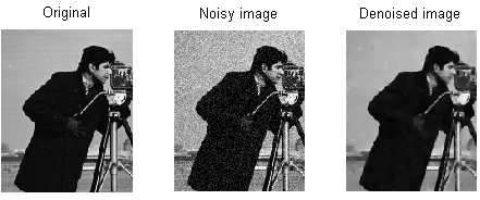
Photo: MAL via Wikimedia Commons, CC BY SA 3.0 (https://en.wikipedia.org/wiki/File:ROF_Denoising_Example.png)
Denoising autoencoders introduce noise into the encoding, resulting in an encoding that is a corrupted version of the original input data. This corrupted version of the data is used to train the model, but the loss function compares the output values with the original input and not the corrupted input. The goal is that the network will be able to reproduce the original, non-corrupted version of the image. By comparing the corrupted data with the original data, the network learns which features of the data are most important and which features are unimportant/corruptions. In other words, in order for a model to denoise the corrupted images, it has to have extracted the important features of the image data.
Variational
Variational autoencoders operate by making assumptions about how the latent variables of the data are distributed. A variational autoencoder produces a probability distribution for the different features of the training images/the latent attributes. When training, the encoder creates latent distributions for the different features of the input images.

When training the network, the encoded data is analyzed and the recognition model outputs two vectors, drawing out the mean and standard deviation of the images. A distribution is created based on these values. This is done for the different latent states. The decoder then takes random samples from the corresponding distribution and uses them to reconstruct the initial inputs to the network.
Autoencoder Applications
Autoencoders can be used for a wide variety of applications, but they are typically used for tasks like dimensionality reduction, data denoising, feature extraction, image generation, sequence to sequence prediction, and recommendation systems.
Data denoising is the use of autoencoders to strip grain/noise from images. Similarly, autoencoders can be used to repair other types of image damage, like blurry images or images missing sections. Dimensionality reduction can help high capacity networks learn useful features of images, meaning the autoencoders can be used to augment the training of other types of neural networks. This is also true of using autoencoders for feature extraction, as autoencoders can be used to identify features of other training datasets to train other models.
In terms of image generation, autoencoders can be used to generate fake human images or animated characters, which has applications in designing face recognition systems or automating certain aspects of animation.
Sequence to sequence prediction models can be used to determine the temporal structure of data, meaning that an autoencoder can be used to generate the next even in a sequence. For this reason, an autoencoder could be used to generate videos. Finally, deep autoencoders can be used to create recommendation systems by picking up on patterns relating to user interest, with the encoder analyzing user engagement data and the decoder creating recommendations that fit the established patterns.


