What is Backpropagation?

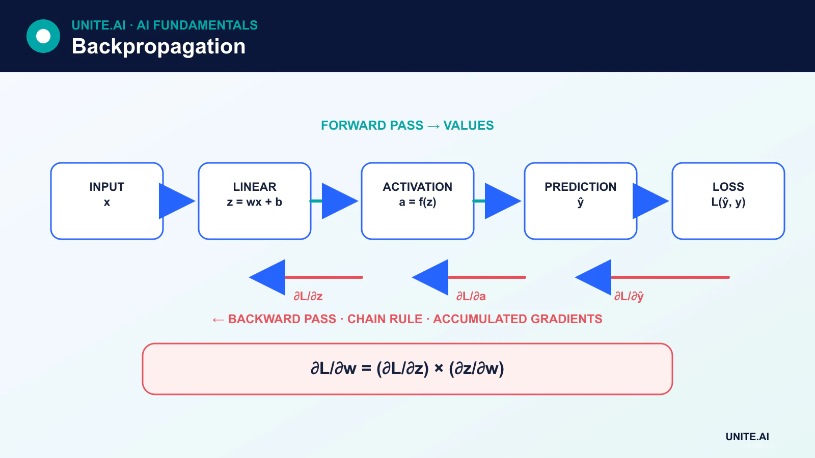
Backpropagation is the algorithm used to compute how a neural network’s loss changes with respect to its trainable parameters. It applies the calculus chain rule backward through the operations recorded during a forward pass.

Backpropagation computes gradients; it does not, by itself, decide the update. An optimizer such as stochastic gradient descent or AdamW uses those gradients to change weights, biases, and other trainable parameters.

Key takeaways

• The forward pass builds intermediate values and produces a prediction.
• The loss function converts the prediction and target into a scalar training objective.
• Backpropagation uses local derivatives and the chain rule to calculate parameter gradients efficiently.
• Modern frameworks implement reverse-mode automatic differentiation over a computational graph.

The forward pass

Consider a simple unit:

z = wx + b
ŷ = activation(z)

The input is x, while w and b are trainable weight and bias parameters. Biases normally change during training just as weights do. A network combines many such operations, plus normalization, attention, convolutions, residual connections, or other differentiable blocks.

The forward pass evaluates those operations and produces a prediction. A loss such as cross-entropy or mean squared error measures the objective. The best loss depends on the task and output interpretation.

The chain rule

If the loss L depends on an intermediate value z, and z depends on parameter w, the chain rule gives:

∂L/∂w = (∂L/∂z) × (∂z/∂w)

A deep network contains many paths. Backpropagation traverses the computational graph in reverse, accumulating contributions when a value affects the loss through more than one path. The result is a gradient for every trainable parameter that participated in the forward computation.

A small numerical example

Suppose ŷ = wx + b, with x = 2, w = 3, and b = 1. The prediction is 7. If the target is 5 and the loss is L = ½(ŷ - y)², then:

• ∂L/∂ŷ = ŷ - y = 2
• ∂ŷ/∂w = x = 2
• ∂L/∂w = 2 × 2 = 4
• ∂L/∂b = 2 × 1 = 2

The optimizer can then move w and b in the negative-gradient direction. This formula is specific to the chosen linear unit and squared-error loss; a universal backpropagation rule is the chain rule over the actual graph, not one fixed “error” equation.

Backpropagation versus gradient descent

Gradient descent is an optimization method. Backpropagation supplies the gradients it needs. A training step usually follows:

1. Clear or reset stored gradients.
2. Run the forward pass.
3. Compute the loss.
4. Run the backward pass.
5. Apply the optimizer update.

Separating these concepts makes it easier to understand momentum, AdamW, gradient accumulation, and mixed-precision training.

Automatic differentiation

Frameworks such as PyTorch record operations and build a graph during the forward pass. Reverse-mode automatic differentiation then calculates vector-Jacobian products efficiently from outputs back to parameters. This is more general than manually coding derivatives for a fixed network and is foundational to modern deep learning frameworks.

Some operations are nondifferentiable or have unstable derivatives. Frameworks define subgradients or documented conventions in certain cases, but practitioners must still understand detached tensors, in-place operations, and numerical precision.

Vanishing and exploding gradients

Repeated multiplication through many layers or time steps can make gradients extremely small or large. Vanishing gradients slow learning in earlier layers; exploding gradients destabilize updates. ReLU-family activations, careful initialization, residual connections, normalization, gated recurrence, and gradient clipping help, but none is a universal cure.

Checking gradients

Finite-difference gradient checking compares an analytical or automatic gradient with a numerical approximation. It is slow but useful for debugging custom operations. Monitoring gradient norms and detecting NaN or infinite values can reveal instability during training.

The chain rule through a computational graph

Backpropagation efficiently computes gradients of a scalar loss with respect to every differentiable parameter. A forward pass records intermediate values in a computational graph. Starting from the loss, reverse-mode automatic differentiation applies the chain rule, multiplying local derivatives and accumulating contributions where paths meet. For a layer y=f(x,w), upstream sensitivity to y combines with partial derivatives to produce sensitivities for x and w. Backpropagation computes gradients; the optimizer decides how parameters change.

A simple affine layer produces y=Wx+b. The gradient for W is the outer product of upstream gradient and input, the gradient for b sums upstream values, and the input gradient multiplies by the transposed weight matrix. Activations add elementwise derivatives. Convolution, normalization, attention, and recurrent reuse follow the same graph principle but require correct tensor shapes, broadcasting, masking, and parameter sharing. Frameworks free saved activations after backward unless retained, so memory often grows with batch, depth, and sequence length.

Gradient failures, verification, and engineering practice

Products of many derivatives can vanish or explode. ReLU-like activations, careful initialization, normalization, residual connections, gating, and gradient clipping address different mechanisms. Saturated activations and nondifferentiable operations can block useful signals; truncated backpropagation limits sequence history; mixed precision can underflow without loss scaling. Exploding gradients are a symptom, so clipping should accompany investigation of learning rate, data, architecture, and numerical errors rather than conceal them.

Verify custom operations with finite-difference gradient checks on small double-precision inputs, avoiding nondifferentiable points. Inspect gradient norms, NaNs, inactive parameters, and whether gradients reach expected modules. Clear accumulated gradients deliberately and distinguish training from evaluation behavior for dropout and normalization. Checkpointing recomputes activations to save memory; distributed training must aggregate gradients consistently. A decreasing training loss shows that an optimization path exists, not that gradients are conceptually correct, data is leakage-free, or the model generalizes.

Worked example: verifying a custom neural layer

An engineer implements a differentiable spectral layer for an audio network. A tiny double-precision test compares automatic gradients with central finite differences across inputs and parameters, excluding points where the operation is intentionally nondifferentiable. Shape, broadcasting, padding, and complex-to-real conversion receive separate cases. The test verifies accumulated gradients when a parameter is reused and confirms that masked audio frames produce no gradient.

During training, dashboards track gradient and activation norms, NaNs, inactive parameters, and loss scaling. A deliberately corrupted batch confirms that validation catches nonfinite output before an optimizer update. Mixed-precision and exported implementations are compared with the reference. Checkpoint resume tests include optimizer state and random order. The layer is not accepted merely because total loss falls; unit gradients, numerical stability, and downstream generalization must all provide consistent evidence.

Implementation evidence and operational readiness

A production decision needs more than a successful demonstration. Define the intended users, operating environment, inputs, outputs, dependencies, owner, and the consequence of each important failure. Establish a reproducible baseline and a versioned evaluation set before tuning. Test ordinary cases, boundary conditions, malformed or missing input, distribution shift, dependency outage, misuse, and the groups or environments most likely to be underserved. Measure task quality together with calibration or uncertainty, latency, throughput, resource cost, accessibility, privacy, and security. Record every transformation and threshold so an independent reviewer can reproduce the result and distinguish evidence from an attractive prototype.

Before launch, assign authority for release, exceptions, changes, rollback, and retirement. Use a staged rollout, preserve a safe fallback, and verify monitoring with deliberately injected failures. Operational telemetry should reveal input quality, output behavior, model or rule version, dependency health, human overrides, and confirmed outcomes without collecting unnecessary sensitive data. Define alert thresholds and a response owner, then review real-world evidence after deployment rather than assuming offline performance will persist. Reevaluate whenever data sources, users, models, vendors, policies, hardware, or objectives change. A maintained system also needs documented recovery, incident learning, deletion and retention procedures, and a clear point at which it should be disabled or replaced.

Frequently asked questions

Does backpropagation update the weights?

Backpropagation calculates gradients. The optimizer applies an update using those gradients, its learning rate, and possibly state such as momentum or adaptive moments.

Is backpropagation biologically realistic?

Standard backpropagation is an engineering algorithm and is not accepted as a detailed model of learning in biological brains. The historical neural analogy should not be treated as biological equivalence.

Primary references

• PyTorch: Autograd mechanics
• PyTorch: The Fundamentals of Autograd
• Rumelhart, Hinton, and Williams: Learning representations by back-propagating errors