What are RNNs and LSTMs in Deep Learning?

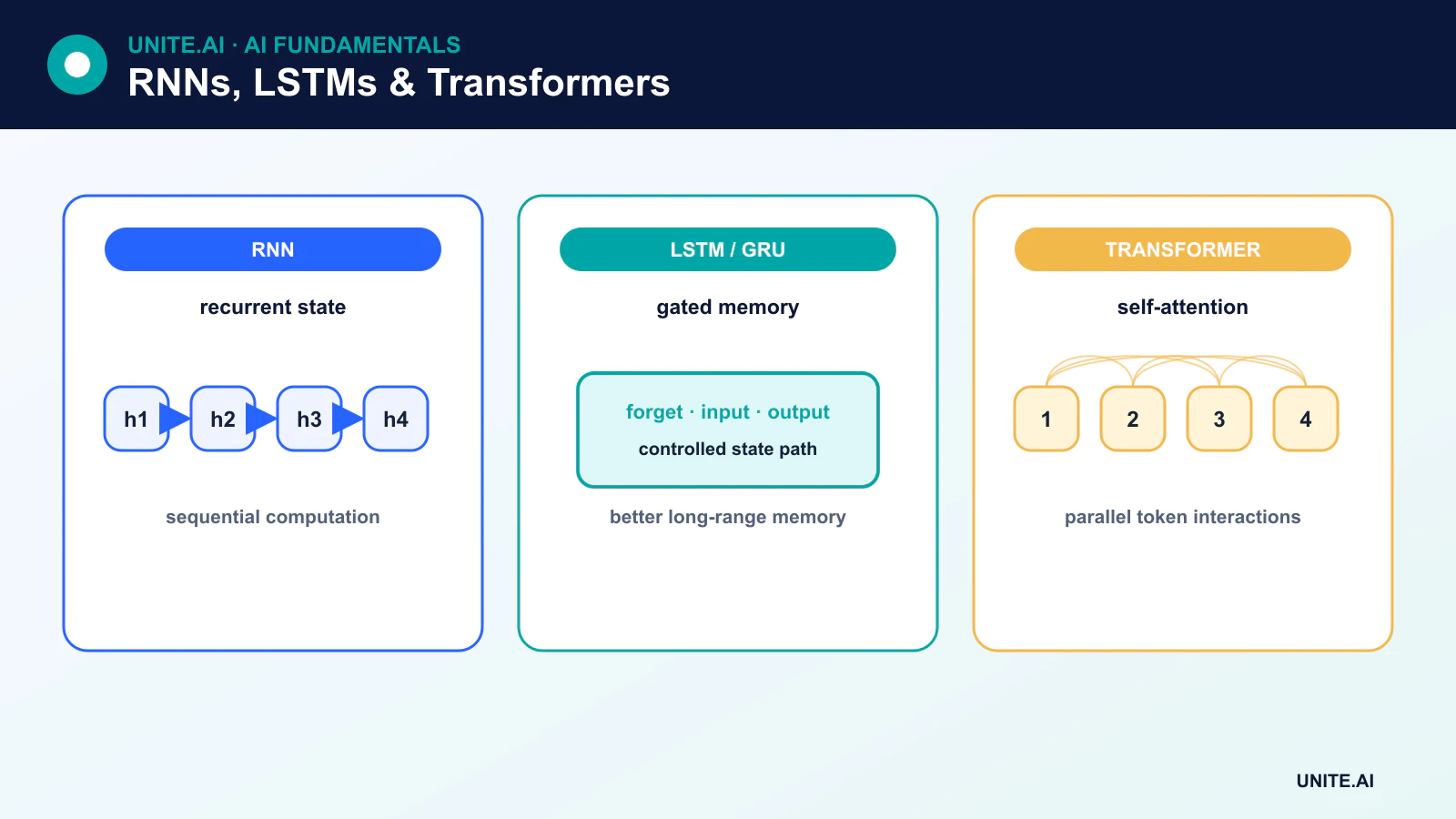
Recurrent neural networks (RNNs) process sequences by updating a hidden state over time. Long short-term memory (LSTM) networks are gated RNNs designed to preserve and control information more effectively than a basic recurrent unit.

RNNs and LSTMs once dominated many language tasks, but modern large chatbots are primarily based on transformers. Recurrent models remain useful for streaming, time-series, speech, control, and resource-constrained systems where incremental state and low latency matter.

Key takeaways

• An RNN reuses the same parameters at every sequence step and carries a hidden state forward.
• Training through time can create vanishing or exploding gradients.
• An LSTM adds a cell state and input, forget, and output gates.
• Transformers handle long-range relationships and parallel training differently; neither architecture is best for every deployment.

How a basic RNN works

At step t, a simple recurrent unit combines the current input xₜ with the previous hidden state hₜ₋₁:

hₜ = activation(Wₓxₜ + Wₕhₜ₋₁ + b)

The hidden state is a learned summary used for the next step and, depending on the task, an output. An “unrolled” diagram draws one copy per time step, but all copies share parameters. The output is not simply copied back as a new raw input; the recurrence passes hidden state through a defined transformation.

Backpropagation through time

RNNs are trained with backpropagation through time (BPTT). The unrolled sequence forms a deep computational graph, and backpropagation calculates how the loss depends on shared recurrent parameters.

Repeated multiplication can make gradients shrink toward zero or grow without bound. Vanishing gradients prevent learning long dependencies; exploding gradients create unstable updates. Gradient clipping addresses exploding gradients, while gating, initialization, normalization, and shorter training windows can help.

Inside an LSTM cell

An LSTM maintains a cell state cₜ in addition to hidden state hₜ. Its gates are learned, data-dependent controls:

• The forget gate controls how much previous cell state is retained.
• The input gate controls how much candidate information is written.
• The output gate controls how much cell information contributes to the hidden state.

Sigmoid outputs between zero and one act as soft gates, while a tanh-transformed candidate supplies new content. The additive cell-state path helps gradients persist, but LSTMs do not guarantee unlimited memory or eliminate all optimization problems.

GRUs and bidirectional recurrence

A gated recurrent unit (GRU) combines gating mechanisms into a simpler recurrent cell without a separate LSTM-style cell state. GRUs can train faster and perform similarly on some tasks.

A bidirectional RNN processes a completed sequence in both directions and combines the states. It can use future context for tagging or encoding, but it is inappropriate for causal streaming when future inputs are not yet available.

Sequence-to-sequence models

Encoder-decoder RNNs map one sequence to another. Attention was introduced to let a decoder consult different encoder states instead of relying on one fixed vector. This line of work led to the transformer architecture, which replaced recurrence with attention-based blocks.

RNNs versus transformers

Transformers process training positions in parallel and create short attention paths between distant tokens. RNNs process state sequentially, limiting parallelism but offering constant-size recurrent state during streaming. Transformer inference may need a growing key-value cache, while an RNN compresses history into its hidden state and can lose detail.

Choose based on sequence length, data scale, hardware, latency, memory, and whether the task is offline or streaming. Hybrid and state-space architectures provide additional tradeoffs.

Current use cases

RNNs and LSTMs remain relevant to forecasting, anomaly detection, sensor processing, speech components, handwriting, embedded control, and low-latency sequence modeling. They are not the default explanation for current large language models or AI chatbots.

Recurrence, gates, and sequence memory

A recurrent neural network processes a sequence by combining the current input with a hidden state carried from previous steps. Shared weights allow variable sequence length, and unrolling exposes the computation through time for training. Basic RNNs can represent temporal dependence but gradients repeatedly multiplied across long sequences tend to vanish or explode. Truncated backpropagation limits memory and compute, while gradient clipping controls extreme updates. The hidden state is a learned summary, not a faithful storage of every earlier token.

Long short-term memory networks add a cell state and input, forget, and output gates that regulate writing, retaining, and exposing information. Gated recurrent units use a simpler reset and update structure. Bidirectional variants use future context and therefore cannot stream causally without delay. Stacked, residual, and attention-augmented recurrent models add capacity. Padding and masks must prevent artificial sequence elements from affecting state or loss, and state should be reset at true sequence boundaries to avoid leakage between examples.

Training, comparison, and stateful serving

RNNs and LSTMs remain useful for streaming, compact on-device models, time series, and workloads where sequential state is efficient. Transformers parallelize training and model long-range interactions differently but can require larger memory and cache. Compare architectures on accuracy, latency, throughput, memory, power, and performance as sequence length changes. Evaluate forecasting with rolling time splits, language with sequence-aware metrics, and anomaly detection with event-level measures. Inspect failure after long gaps, regime changes, missing samples, and abrupt sequence boundaries.

Stateful deployment must associate hidden state with the correct session, expire it, encrypt it if sensitive, and reset it after errors or model changes. Out-of-order or duplicated events can corrupt state; include timestamps, sequence numbers, and idempotency. Monitor state age, sequence length, missingness, output drift, and latency. Quantization needs gate-sensitive validation because small numeric changes can accumulate over time. RNN memory enables context, but it can also preserve private or stale information, so retention and user controls belong in the design.

Worked example: an LSTM for streaming sensor sequences

A utility uses an LSTM to forecast short-term load from recent measurements, calendar, and weather. Sequences are built with strict time order; hidden state resets at feeder boundaries, and padding is masked. Seasonal-naive and gradient-boosted baselines are compared with the LSTM across rolling windows. Tests cover missing intervals, delayed weather, holidays, outages, and sequence lengths beyond typical training.

The streaming service associates state with one feeder, rejects out-of-order duplicates, and expires state after long gaps or model updates. A safe statistical forecast replaces output when sensors or state are invalid. Quantized inference is checked over long sequences for accumulated drift. Monitoring tracks state age, missingness, latency, bias, and interval error. The model is retrained only after grid changes and reviewed outcomes show that the learned temporal relationships no longer generalize.

Implementation evidence and operational readiness

A production decision needs more than a successful demonstration. Define the intended users, operating environment, inputs, outputs, dependencies, owner, and the consequence of each important failure. Establish a reproducible baseline and a versioned evaluation set before tuning. Test ordinary cases, boundary conditions, malformed or missing input, distribution shift, dependency outage, misuse, and the groups or environments most likely to be underserved. Measure task quality together with calibration or uncertainty, latency, throughput, resource cost, accessibility, privacy, and security. Record every transformation and threshold so an independent reviewer can reproduce the result and distinguish evidence from an attractive prototype.

Before launch, assign authority for release, exceptions, changes, rollback, and retirement. Use a staged rollout, preserve a safe fallback, and verify monitoring with deliberately injected failures. Operational telemetry should reveal input quality, output behavior, model or rule version, dependency health, human overrides, and confirmed outcomes without collecting unnecessary sensitive data. Define alert thresholds and a response owner, then review real-world evidence after deployment rather than assuming offline performance will persist. Reevaluate whenever data sources, users, models, vendors, policies, hardware, or objectives change. A maintained system also needs documented recovery, incident learning, deletion and retention procedures, and a clear point at which it should be disabled or replaced.

Frequently asked questions

Is an LSTM always better than a basic RNN?

No. Gating helps many long-dependency problems but adds computation and parameters. A basic RNN can be adequate for short, simple sequences, and another architecture may be better for very long context.

Can an LSTM process an unlimited history?

No. Its state has finite capacity, gradients and training data impose limits, and relevant details can be overwritten. Long-context performance must be measured rather than inferred from the architecture’s name.

Primary references

• Hochreiter and Schmidhuber: Long Short-Term Memory
• PyTorch: LSTM
• Vaswani et al.: Attention Is All You Need