What is a Confusion Matrix?

A confusion matrix is a table that counts how often a classifier’s predictions agree or disagree with known labels. It reveals which classes are being confused and provides the counts used to calculate metrics such as precision, recall, specificity, and F1. It is one of the core diagnostic tools for supervised learning classification problems.

The matrix itself is not a single performance score. It is a structured view of outcomes at a particular decision threshold, dataset, and class definition.

Key takeaways

• For binary classification, the four outcomes are true positive, false positive, false negative, and true negative.
• Always label the axes: libraries and publications do not all place actual and predicted classes in the same orientation.
• Accuracy can hide serious errors when classes are imbalanced.
• Changing the classification threshold changes the confusion matrix and the tradeoff between precision and recall.

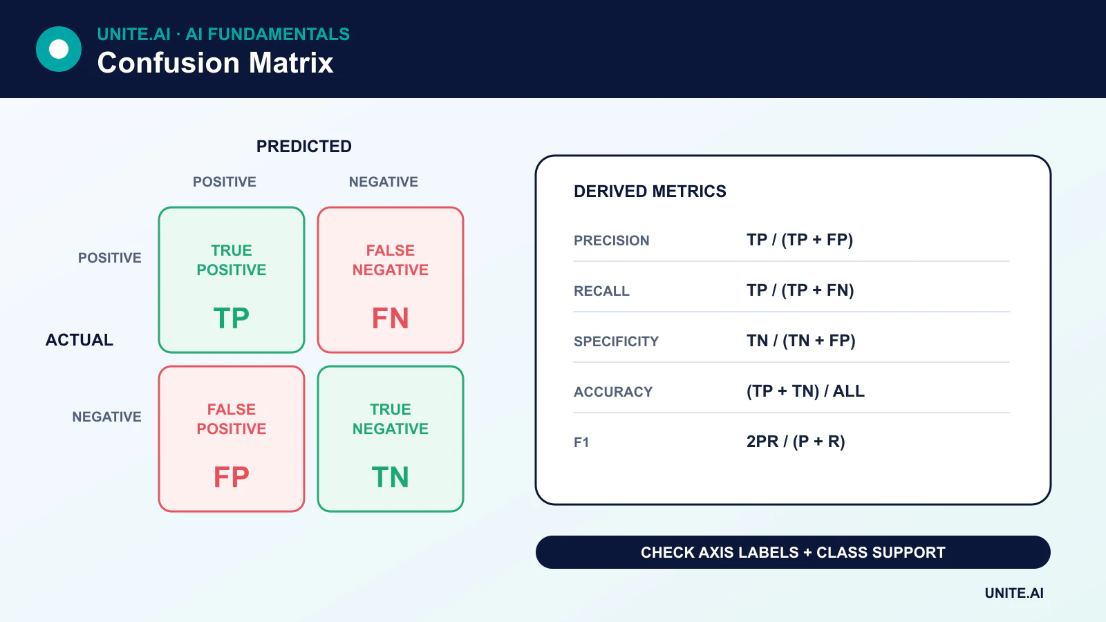
The four binary-classification outcomes

• True positive (TP): the example is positive and the model predicts positive.
• False positive (FP): the example is negative but the model predicts positive.
• False negative (FN): the example is positive but the model predicts negative.
• True negative (TN): the example is negative and the model predicts negative.

In scikit-learn’s convention, rows are true classes and columns are predicted classes. Other visualizations may transpose this arrangement, so the labels—not the corner positions—should guide interpretation.

Metrics derived from a confusion matrix

Precision

Precision = TP / (TP + FP)

Precision answers: among examples predicted positive, what proportion was actually positive?

Recall or sensitivity

Recall = TP / (TP + FN)

Recall answers: among all actual positive examples, what proportion did the model identify? In binary classification, positive-class recall is also called sensitivity or the true-positive rate.

Specificity

Specificity = TN / (TN + FP)

Specificity is recall for the negative class: among actual negatives, what proportion did the model correctly reject?

Accuracy

Accuracy = (TP + TN) / (TP + TN + FP + FN)

Accuracy is useful when classes and error costs are reasonably balanced. It can be deceptive when one class dominates.

F1 score

F1 = 2 × (Precision × Recall) / (Precision + Recall)

F1 summarizes precision and recall with a harmonic mean. It ignores true negatives, so it is not the right summary for every task.

A worked example

Suppose a test set contains 1,000 transactions. Fifty are fraudulent. A model finds 40 of those frauds but flags 30 legitimate transactions:

• TP = 40
• FN = 10
• FP = 30
• TN = 920

The model has 96% accuracy, but its precision is about 57% and recall is 80%. The high accuracy is driven largely by the many legitimate transactions. Whether this model is acceptable depends on the cost of missed fraud, investigation capacity, and how calibrated its risk scores are.

Thresholds change the matrix

Many classifiers output a score rather than an unavoidable yes/no answer. Lowering the positive threshold generally increases recall and false positives; raising it generally increases precision or specificity while missing more positives. The threshold should be chosen using validation data and real error costs, not automatically fixed at 0.5.

Precision-recall and ROC curves summarize performance across thresholds. Precision-recall curves are often more informative when the positive class is rare.

Multiclass confusion matrices

For K classes, the matrix is K × K. Correct predictions lie on the diagonal; off-diagonal cells show which class pairs are confused. Per-class metrics can be averaged in different ways:

• Macro average: gives each class equal weight.
• Weighted average: weights each class by its number of examples.
• Micro average: aggregates outcome counts before calculating the metric.

Reporting only one average can hide poor performance on smaller classes. Include support counts and per-class results where the differences matter.

Common mistakes

• Reading a transposed matrix without checking axis labels.
• Calculating metrics from training data instead of an appropriate held-out set.
• Ignoring class prevalence, sampling strategy, or duplicate entities across splits.
• Comparing matrices produced at different thresholds without noting the change.
• Treating all false positives and false negatives as equally costly.

A confusion matrix is therefore a diagnostic tool, not a complete evaluation. Calibration, subgroup analysis, robustness, and downstream consequences also belong in a classification review.

Reading every cell and deriving useful metrics

For binary classification, the confusion matrix counts true positives, false positives, false negatives, and true negatives for a chosen positive class and threshold. Accuracy divides correct predictions by all cases; precision asks what fraction of predicted positives were correct; recall asks what fraction of actual positives were found; specificity measures actual negatives correctly rejected. F1 is the harmonic mean of precision and recall. None is inherently best: fraud screening, medical triage, and spam filtering assign different consequences to the same cells.

For multiclass problems, rows commonly represent actual classes and columns predicted classes, though conventions vary, so labels must be explicit. One-vs-rest counts produce per-class precision and recall. Macro averaging weights classes equally; micro averaging aggregates decisions and favors common classes; weighted averaging follows class support. Multilabel tasks allow several labels per item and need label-wise or sample-wise definitions. Normalize by row to inspect recall patterns or by column to inspect prediction composition, but retain raw counts so rare groups are not visually exaggerated.

Thresholds, uncertainty, and operational decisions

A confusion matrix summarizes hard decisions at one threshold. Use precision–recall or ROC curves to compare thresholds, then select an operating point from capacity, prevalence, and error cost. Calibration asks whether predicted probabilities match observed frequency and is separate from ranking. When prevalence changes, precision can change even if sensitivity and specificity remain stable. Report confidence intervals or bootstrap variation, and avoid drawing conclusions from a handful of errors in a small subgroup.

Audit matrices by time, location, device, language, and relevant affected groups to find concentrated errors. Compare the model with the existing decision process, including human review. For cascades, record errors at each stage: retrieval, classification, thresholding, and action. Monitor live outcome labels with their delay and correction process. A seemingly improved F1 can still increase harmful false negatives or exceed review capacity. The confusion matrix is a decision ledger; connect every cell to who experiences the error and what response follows.

Worked example: selecting a medical-screening threshold

A machine-learning screening model outputs a risk score for a condition with low prevalence. The team creates confusion matrices across thresholds and reports sensitivity, specificity, precision, false referrals, and missed cases with confidence intervals. Because positive predictive value depends on prevalence, it models the intended population rather than quoting one dataset’s precision. Results are segmented by device, site, age, sex, and other clinically justified groups.

Clinicians choose an operating point that preserves required sensitivity without overwhelming confirmatory testing. The matrix is translated into expected counts per 10,000 screened people so consequences are understandable. Scores outside validated conditions produce no automated conclusion. Monitoring compares predictions with delayed confirmed diagnoses, tracks capacity and calibration, and triggers review when prevalence or acquisition changes. The confusion matrix remains linked to the exact model, threshold, and population.

Implementation evidence and operational readiness

A production decision needs more than a successful demonstration. Define the intended users, operating environment, inputs, outputs, dependencies, owner, and the consequence of each important failure. Establish a reproducible baseline and a versioned evaluation set before tuning. Test ordinary cases, boundary conditions, malformed or missing input, distribution shift, dependency outage, misuse, and the groups or environments most likely to be underserved. Measure task quality together with calibration or uncertainty, latency, throughput, resource cost, accessibility, privacy, and security. Record every transformation and threshold so an independent reviewer can reproduce the result and distinguish evidence from an attractive prototype.

Before launch, assign authority for release, exceptions, changes, rollback, and retirement. Use a staged rollout, preserve a safe fallback, and verify monitoring with deliberately injected failures. Operational telemetry should reveal input quality, output behavior, model or rule version, dependency health, human overrides, and confirmed outcomes without collecting unnecessary sensitive data. Define alert thresholds and a response owner, then review real-world evidence after deployment rather than assuming offline performance will persist. Reevaluate whenever data sources, users, models, vendors, policies, hardware, or objectives change. A maintained system also needs documented recovery, incident learning, deletion and retention procedures, and a clear point at which it should be disabled or replaced.

Frequently asked questions

What is a normalized confusion matrix?

Normalization divides counts by the true-class total, predicted-class total, or all observations. It makes rates easier to compare across classes, but the report should also retain raw support counts so small groups are not mistaken for equally large ones.

Can a confusion matrix evaluate regression?

Not directly. A confusion matrix requires discrete classes. Binning a continuous target discards information; regression should normally use residual analysis and metrics designed for continuous values, such as MAE or RMSE.

Primary references

• scikit-learn: confusion_matrix
• scikit-learn: Metrics and scoring
• scikit-learn: classification_report