What is Gradient Descent?

Gradient descent is an optimization method that adjusts model parameters to reduce an objective function. In neural-network training, that objective is usually a loss calculated over examples. The gradient points in the direction of steepest local increase, so gradient descent takes a step in the opposite direction.

The gradient describes local sensitivity; its magnitude is not a direct measurement of how fast a model is “learning.” Actual progress also depends on the learning rate, curvature, noise, parameterization, optimizer state, and data.

Key takeaways

• Backpropagation computes gradients, while gradient descent uses them to update parameters.
• Mini-batch optimization is the standard practical approach for deep learning.
• The learning rate controls update scale and may follow a schedule rather than shrinking after every step.
• Momentum, AdamW, clipping, and normalization address different optimization problems.

The basic update rule

For parameter vector θ, learning rate η, and loss L:

θ ← θ - η∇L(θ)

The gradient ∇L(θ) contains one partial derivative per parameter. Subtracting it moves downhill locally. A stationary point has gradient zero, but it may be a minimum, maximum, saddle point, or flat region. Deep-learning loss surfaces are nonconvex, so training is not guaranteed to find a unique global minimum or zero loss.

Batch, stochastic, and mini-batch methods

Batch gradient descent

Batch gradient descent calculates a gradient using the full training set for every update. The estimate is stable but can be expensive in time and memory, and one update may underuse modern accelerators.

Stochastic gradient descent

Strict stochastic gradient descent uses one randomly selected example per update. Its gradients are noisy, which can help exploration of the loss surface, but single-example operations may be inefficient on parallel hardware.

Mini-batch gradient descent

Mini-batch training estimates the gradient from a subset of examples. It balances statistical noise with efficient matrix operations and is the usual approach in deep learning. Batch size affects memory, throughput, gradient noise, normalization, and sometimes generalization.

Choosing a learning rate

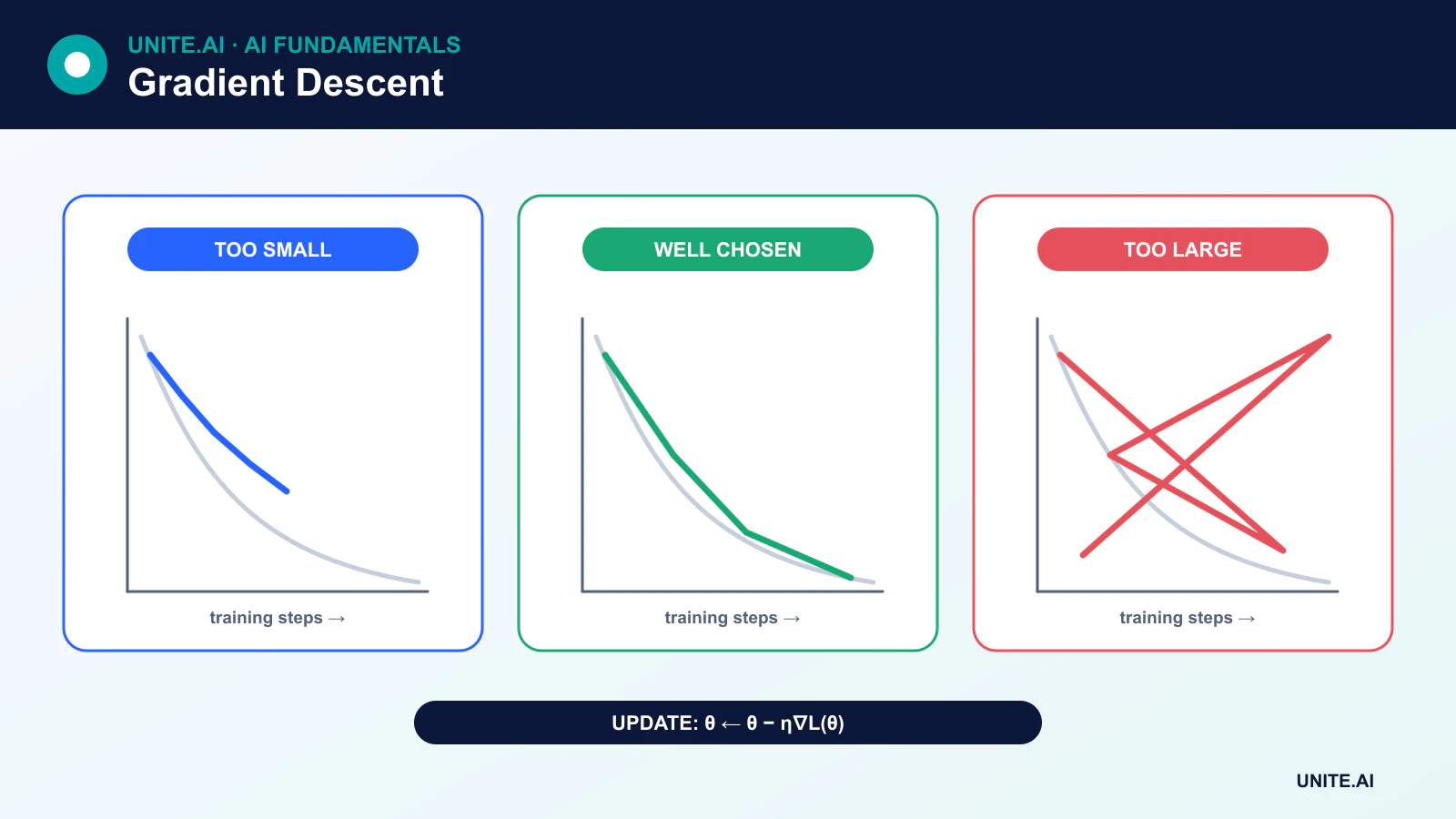
A rate that is too large can overshoot useful regions or cause divergence. A rate that is too small may make training impractically slow or stall in flat regions. The best scale depends on the optimizer, batch size, model, initialization, and objective.

Schedules can warm up gradually, decay at milestones, follow a cosine curve, or respond to validation progress. The rate does not have to shrink monotonically after every update. Warm restarts and cyclical schedules deliberately increase it during parts of training.

Momentum

Momentum maintains an exponential moving average of past gradients. It can accelerate progress along consistent directions and reduce oscillation across steep, narrow directions. Nesterov-style momentum evaluates or approximates the gradient after looking ahead along the momentum direction.

Adaptive optimizers

RMSProp scales updates using a moving average of squared gradients. Adam combines momentum-like first moments with second-moment scaling. AdamW decouples weight decay from the adaptive gradient update and is widely used for transformers.

Adaptive optimizers often make early training easier, but they are not automatically superior for every model or final generalization target. Optimizer comparisons need matched schedules and careful tuning.

Gradient clipping and accumulation

Gradient clipping caps a gradient’s norm or values to reduce the impact of exploding gradients, especially in recurrent or unstable training. Gradient accumulation adds gradients across several smaller batches before an update, approximating a larger effective batch when memory is limited.

Monitoring optimization

Track training and validation loss, task metrics, learning rate, gradient norms, parameter norms, and numerical errors. Falling training loss with worsening validation performance indicates overfitting, not an optimization success that should automatically continue.

Optimization minimizes the objective it is given. A low loss does not prove that the data, metric, or real-world behavior is appropriate. Leakage, poor labels, and a misaligned objective can produce a well-optimized but harmful model.

Optimization geometry and update rules

Gradient descent updates parameters opposite the gradient of a loss. Full-batch descent uses every training example per step; stochastic descent uses one; mini-batch methods estimate the gradient from a subset and dominate deep learning. The learning rate sets step scale. Too small wastes computation or stalls; too large oscillates or diverges. Momentum accumulates a moving direction, while adaptive methods such as Adam scale coordinates using gradient moments. Their different implicit biases can produce models with similar training loss but different generalization.

Loss surfaces in neural networks contain flat and sharp regions, saddles, symmetries, and poorly conditioned directions. Feature scaling, normalization, initialization, residual connections, and preconditioning change the geometry seen by the optimizer. Schedules can warm up, decay, cycle, or react to plateaus. Weight decay is distinct from merely adding an L2 penalty in some adaptive optimizers. Batch size affects noise, memory, parallelism, and the learning-rate regime, so optimizer comparisons need matched training budgets and careful tuning.

Diagnosis, reproducibility, and stopping

Track training and validation loss, task metrics, gradient and parameter norms, learning rate, throughput, and numerical warnings. Divergence can come from corrupt batches, invalid labels, unstable mixed precision, or an incorrect loss reduction. Plateaus may indicate under-capacity, saturated activations, poor features, excessive regularization, or a schedule issue. Overfitting needs data, augmentation, regularization, or early stopping—not a claim that the optimizer failed. Inspect representative errors and compare a simple baseline before increasing training complexity.

Reproducibility requires seeds, data order, code, configuration, hardware and library versions, though some accelerator kernels remain nondeterministic. Save checkpoints with optimizer and scheduler state so training can resume consistently. Select a checkpoint on validation criteria fixed in advance and reserve an untouched test set. In distributed training, confirm effective batch size, gradient averaging, and handling of failed workers. Optimization minimizes the chosen objective on available data; it does not ensure calibrated probabilities, causal reasoning, fairness, safety, or real-world utility.

Worked example: tuning an optimizer for a language model

A team fixes tokenizer, data order, model, effective batch, and training-token budget, then compares SGD with momentum and AdamW across defensible learning-rate schedules. Warm-up, decay, weight decay, clipping, and precision are logged. Each candidate runs several seeds, and validation uses a held-out time slice plus task evaluations. Throughput and energy are reported alongside loss so a slightly better optimizer is not selected at disproportionate cost.

Diagnostics reveal whether instability originates in one data shard, excessive step size, underflow, or model architecture. Checkpoints preserve optimizer and scheduler state and are resumed in a test. The final choice is based on validation quality and robustness, not the lowest training loss. A sealed test set is run once after selection. Production inference is separately calibrated and monitored because optimizer success during pretraining does not establish safe or truthful behavior.

Implementation evidence and operational readiness

A production decision needs more than a successful demonstration. Define the intended users, operating environment, inputs, outputs, dependencies, owner, and the consequence of each important failure. Establish a reproducible baseline and a versioned evaluation set before tuning. Test ordinary cases, boundary conditions, malformed or missing input, distribution shift, dependency outage, misuse, and the groups or environments most likely to be underserved. Measure task quality together with calibration or uncertainty, latency, throughput, resource cost, accessibility, privacy, and security. Record every transformation and threshold so an independent reviewer can reproduce the result and distinguish evidence from an attractive prototype.

Before launch, assign authority for release, exceptions, changes, rollback, and retirement. Use a staged rollout, preserve a safe fallback, and verify monitoring with deliberately injected failures. Operational telemetry should reveal input quality, output behavior, model or rule version, dependency health, human overrides, and confirmed outcomes without collecting unnecessary sensitive data. Define alert thresholds and a response owner, then review real-world evidence after deployment rather than assuming offline performance will persist. Reevaluate whenever data sources, users, models, vendors, policies, hardware, or objectives change. A maintained system also needs documented recovery, incident learning, deletion and retention procedures, and a clear point at which it should be disabled or replaced.

Frequently asked questions

Does gradient descent always reach the global minimum?

No. For convex objectives, appropriate conditions provide strong guarantees. Deep-network objectives are nonconvex, and practical optimizers usually seek a useful solution rather than prove they found the unique global minimum.

Why can a zero gradient be misleading?

A zero or tiny gradient may indicate a minimum, maximum, saddle point, saturation, or flat plateau. Training diagnostics must consider loss history, curvature, parameter scale, and validation performance.

Primary references

• PyTorch: Optimization algorithms
• Loshchilov and Hutter: Decoupled Weight Decay Regularization