What is Bayes Theorem?

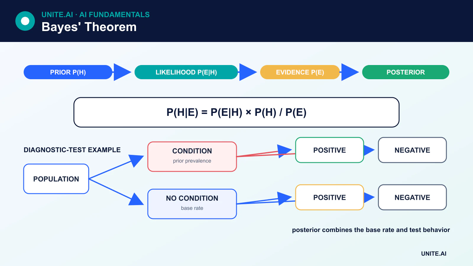
Bayes’ theorem describes how to update the probability of a hypothesis after observing evidence. It connects the probability of evidence given a hypothesis with the probability of the hypothesis given that evidence.

This distinction is central to statistical reasoning and machine learning. A test can be highly accurate when a condition is present while a positive result still has a modest probability of indicating the condition if the condition is rare.

Key takeaways

• The posterior combines a prior belief with the likelihood of observed evidence.
• The evidence term normalizes the possible hypotheses.
• Base rates can dominate apparently strong evidence.
• Naive Bayes assumes features are conditionally independent given the class, not independent in every circumstance.

The formula

P(A|B) = P(B|A)P(A) / P(B)

• P(A) is the prior probability of hypothesis A.
• P(B|A) is the likelihood of observing evidence B if A is true.
• P(B) is the overall probability of the evidence.
• P(A|B) is the posterior probability of A after observing B.

The theorem follows from two equivalent expressions for joint probability: P(A ∩ B) = P(B|A)P(A) and P(A ∩ B) = P(A|B)P(B).

A numerical base-rate example

Suppose a condition affects 1% of a population. A test has 90% sensitivity and a 5% false-positive rate. Consider 1,000 people:

• About 10 have the condition; the test correctly flags 9.
• About 990 do not; a 5% false-positive rate flags roughly 50.
• There are therefore about 59 positive results, of which 9 are true positives.

The probability of the condition after a positive result is about 9 / 59 ≈ 15%, not 90%. The test’s sensitivity answers P(positive | condition); the user usually wants P(condition | positive). Bayes’ theorem connects them using the base rate.

Bayesian updating

As new evidence arrives, a posterior can become the prior for the next update. A complete Bayesian model specifies possible hypotheses, prior distributions, a likelihood, and the quantity to infer. Uncertainty is represented with a posterior distribution rather than only a point estimate.

The prior should be documented and tested for sensitivity. A weakly informative prior can regularize implausible values, while a poorly chosen strong prior can dominate limited data.

Naive Bayes classifiers

Naive Bayes predicts a class y from features x₁ … xₙ using Bayes’ theorem and the assumption:

P(x₁, …, xₙ | y) = Π P(xᵢ | y)

The features are assumed to be conditionally independent after the class is known. This is often unrealistic, yet the classifier can work well when the resulting class scores are still useful.

Common variants

• Multinomial Naive Bayes models count-like features and is common in document classification.
• Bernoulli Naive Bayes models binary feature presence.
• Gaussian Naive Bayes models each continuous feature with a class-conditional Gaussian distribution.
• Categorical Naive Bayes models discrete categories.

Smoothing and numerical stability

If a feature value never appears with a class in training, an unsmoothed probability estimate can become zero and eliminate the entire product. Additive or Laplace-style smoothing prevents this. Implementations calculate log probabilities so multiplying many small values becomes adding stable log values.

Probabilities, scores, and calibration

Naive Bayes probability outputs can be poorly calibrated because correlated features are effectively counted more than once. A classifier may rank classes well while overstating confidence. Calibration should be evaluated on held-out data when probabilities drive decisions.

Bayes beyond Naive Bayes

Bayesian inference supports hierarchical models, A/B tests, scientific parameter estimation, forecasting, uncertainty-aware decision making, and probabilistic graphical models. Approximate methods such as Markov chain Monte Carlo and variational inference are used when a posterior cannot be calculated in closed form.

Common reasoning mistakes

• Confusing P(A|B) with P(B|A).
• Ignoring a rare or common base rate.
• Treating a prior as objective or leaving it undocumented.
• Assuming a high likelihood automatically implies a high posterior.
• Interpreting a predictive association as causation.

Conditional probability, odds, and evidence

Bayes’ theorem relates the probability of a hypothesis after evidence to its prior probability, the likelihood of observing that evidence under the hypothesis, and the total probability of the evidence. In odds form, posterior odds equal prior odds multiplied by a likelihood ratio. This separates what was believed before a test from how strongly the test distinguishes hypotheses. A highly accurate-seeming test can still produce many false positives when the condition is rare because the base rate enters the posterior.

The likelihood is a function of the hypothesis for fixed observed data and should not be confused with the probability of the hypothesis. Evidence normalization sums or integrates across competing hypotheses. Conditional independence assumptions can simplify calculation, as in naive Bayes, but must be checked against consequences. Multiple pieces of evidence cannot be multiplied as independent when they share causes or duplicate information. Causal direction also matters: P(evidence|hypothesis) is not generally P(hypothesis|evidence), the classic inverse-probability error.

Modeling choices, computation, and decision use

Bayesian analysis specifies a prior, likelihood, and posterior predictive distribution. Priors can encode established knowledge, regularize small samples, or be weakly informative; they should be justified and tested through sensitivity analysis. Conjugate models yield analytic updates, while Markov chain Monte Carlo, variational inference, and sequential methods approximate complex posteriors. Diagnose convergence, effective sample size, approximation error, and prior predictive plausibility rather than reporting a posterior number without computation checks.

A posterior probability informs but does not by itself choose an action. Decisions require losses, benefits, constraints, and available alternatives. Evaluate probabilistic models with calibration, proper scoring rules, and posterior predictive checks on new data. Update only with evidence collected under a modeled process; selection bias and dataset shift can invalidate the likelihood. Communicate credible intervals and assumptions without treating them as guaranteed frequency ranges. Bayes’ theorem is exact probability algebra, while the quality of a Bayesian conclusion depends on the model and evidence supplied.

Worked example: interpreting a diagnostic test

A test has 95% sensitivity and 90% specificity, but the condition affects only 1% of the screened population. For 10,000 people, about 95 true positives and 990 false positives are expected, yielding a positive predictive value under 9%. Bayes’ theorem makes the base-rate effect explicit. The calculation states population, test threshold, and uncertainty rather than advertising sensitivity as the chance a positive result is correct. This distinction is also fundamental to careful data science.

Clinicians update probability with additional evidence only when dependence among tests is modeled. A decision threshold incorporates harm of missed disease, confirmatory-test risk, cost, and patient preference. Calibration is checked in the local population, and prevalence changes trigger review. The posterior supports discussion and next steps; it does not replace confirmatory diagnosis. Reporting uses natural frequencies and sensitivity analysis so patients and practitioners can see how the conclusion changes under plausible assumptions.

Implementation evidence and operational readiness

A production decision needs more than a successful demonstration. Define the intended users, operating environment, inputs, outputs, dependencies, owner, and the consequence of each important failure. Establish a reproducible baseline and a versioned evaluation set before tuning. Test ordinary cases, boundary conditions, malformed or missing input, distribution shift, dependency outage, misuse, and the groups or environments most likely to be underserved. Measure task quality together with calibration or uncertainty, latency, throughput, resource cost, accessibility, privacy, and security. Record every transformation and threshold so an independent reviewer can reproduce the result and distinguish evidence from an attractive prototype.

Before launch, assign authority for release, exceptions, changes, rollback, and retirement. Use a staged rollout, preserve a safe fallback, and verify monitoring with deliberately injected failures. Operational telemetry should reveal input quality, output behavior, model or rule version, dependency health, human overrides, and confirmed outcomes without collecting unnecessary sensitive data. Define alert thresholds and a response owner, then review real-world evidence after deployment rather than assuming offline performance will persist. Reevaluate whenever data sources, users, models, vendors, policies, hardware, or objectives change. A maintained system also needs documented recovery, incident learning, deletion and retention procedures, and a clear point at which it should be disabled or replaced.

Frequently asked questions

What is the difference between a likelihood and a probability?

With parameters fixed, a model assigns probability to possible data. With observed data fixed, the same expression can be viewed as a likelihood function over possible parameter values. The numerical formula may match while the interpretation differs.

Is Naive Bayes fully Bayesian inference?

It uses Bayes’ theorem for classification under a strong conditional-independence model. Broader Bayesian inference places distributions over unknown quantities and reasons with a posterior distribution.

Primary references

• scikit-learn: Naive Bayes
• NIST/SEMATECH: Probability distributions and conditional probability