AI Fundamentals
What is Linear Regression?

 Add Unite.AI to your preferred sources on Google

Linear regression models a continuous target as a linear combination of one or more input features. It is used for prediction, estimation, and as a transparent baseline for understanding whether a more complicated model adds meaningful value.
The words independent variable and dependent variable describe roles in the model, not proven cause and effect. A regression can identify an association while confounding, selection bias, reverse causation, or measurement error explains the relationship.
Key takeaways
- The target y is modeled from input features X; the article’s older version reversed these labels in one formula explanation.
- Ordinary least squares minimizes the sum of squared residuals.
- Residual diagnostics and assumptions matter for inference and uncertainty.
- Ridge and lasso regularization help when predictors are numerous or correlated.
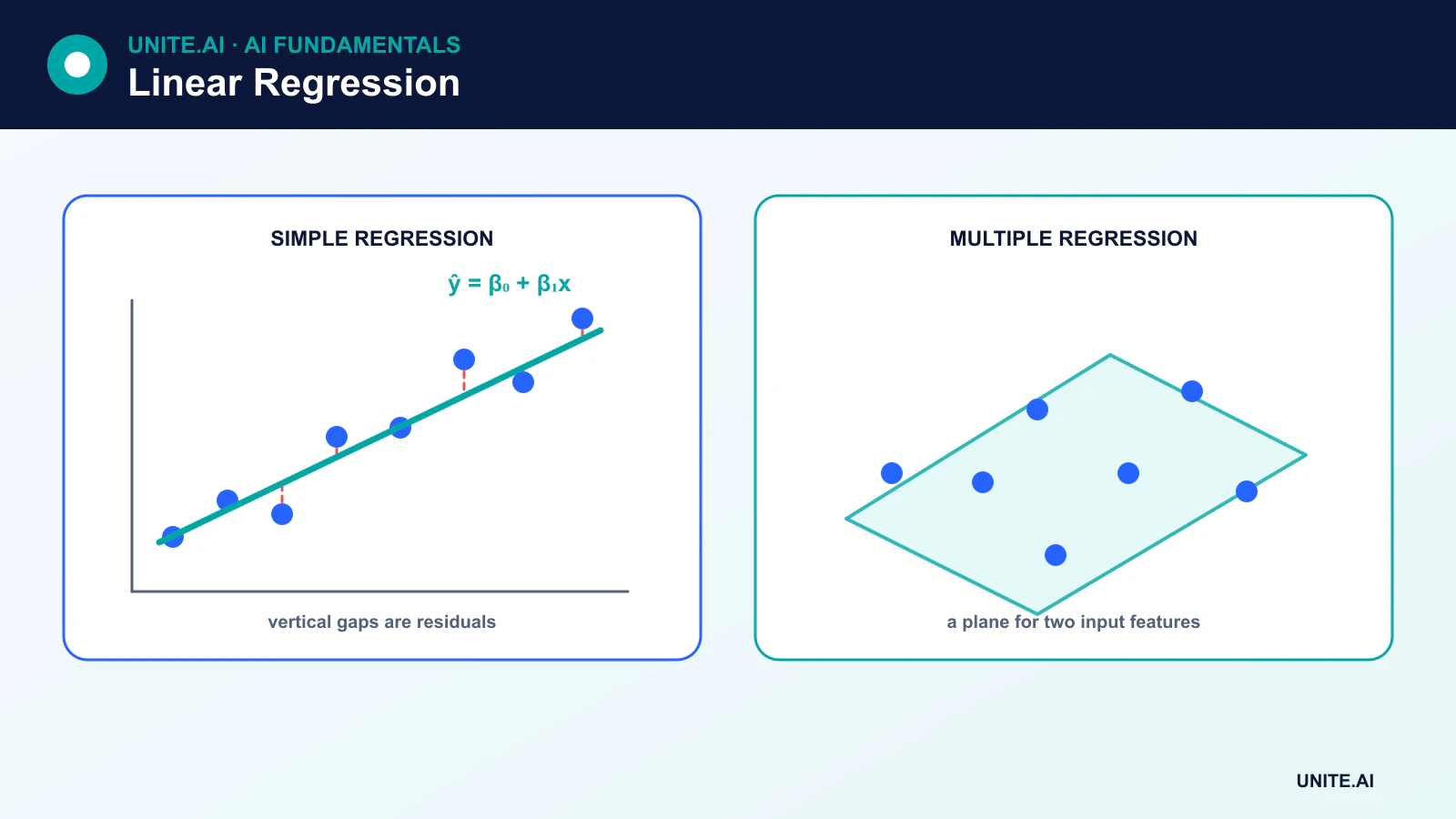
Simple linear regression
With one feature, the model is:
ŷ = β₀ + β₁x
β₀ is the intercept and β₁ is the slope. The residual for observation i is yᵢ - ŷᵢ. Ordinary least squares (OLS) chooses coefficients that minimize the sum of squared residuals.
The slope estimates the expected change in the target associated with a one-unit change in the feature under the fitted model. It should not be described as a causal effect unless the study design and assumptions support causal identification.
Multiple linear regression
With p features:
ŷ = β₀ + β₁x₁ + β₂x₂ + … + βₚxₚ
Each coefficient is interpreted conditional on the other included features. Multiple regression can incorporate categorical variables through encoding, polynomial terms, and interactions. It remains “linear” because it is linear in the coefficients, even if transformed features such as x² are included.
Assumptions and diagnostics
For prediction, the core question is how well the model generalizes. For classical coefficient tests and intervals, additional assumptions become important:
- Linearity: the conditional mean is represented by the chosen linear form.
- Independent or correctly modeled errors: repeated, grouped, spatial, or time-series observations may require a different error structure.
- Constant error variance: heteroscedasticity affects standard errors and uncertainty estimates.
- Limited multicollinearity: strongly correlated predictors make individual coefficients unstable.
- Residual distribution: normality is relevant to some small-sample inference, not a requirement that every feature be normally distributed.
Residual plots, leverage and influence measures, and domain review can identify outliers, nonlinearity, changing variance, or observations that dominate the fit.
Evaluating predictions
- Mean absolute error (MAE) averages absolute residual size.
- Mean squared error (MSE) gives larger errors more weight.
- Root mean squared error (RMSE) returns squared error to target units.
- R² compares residual variation with a constant baseline on the evaluated data.
R² is not accuracy, does not establish causation, and can be negative on held-out data. Validation should match the real prediction setting, including time or group-aware splits when necessary.
Ridge, lasso, and elastic net
Ridge regression adds an L2 penalty that shrinks coefficients and stabilizes correlated predictors. Lasso adds an L1 penalty and can set coefficients to zero. Elastic net combines both. Features usually need compatible scaling before these penalties are compared.
Regularization introduces bias in exchange for lower variance and can reduce overfitting. The penalty strength is selected with validation, not the final test set.
When linear regression is the wrong tool
A linear model may fail when relationships are strongly nonlinear, errors depend on past values, target distributions require specialized modeling, or a few outliers dominate squared loss. Decision trees, generalized linear models, time-series models, robust regression, or nonlinear methods may fit better.
Even when a complex model wins, linear regression remains a valuable baseline. If a large system cannot outperform it reliably, the added complexity may not be justified.
Model assumptions, estimation, and diagnostics
Linear regression models the conditional mean of a numeric outcome as an intercept plus weighted predictors. Ordinary least squares chooses coefficients that minimize squared residuals. Coefficients describe the expected outcome change for one-unit predictor change while other included variables are held constant, under the specified model. This is an association unless causal identification assumptions and study design justify more. Units, coding, transformations, interactions, and reference categories determine interpretation, so coefficients without a data dictionary are incomplete.
Classical inference relies on assumptions about functional form, independent errors, constant variance, and error distribution for particular tests and intervals. Residual-versus-fitted plots reveal nonlinearity or heteroscedasticity; Q–Q plots assess tail behavior; leverage and influence diagnostics identify observations that strongly affect estimates. Correlated predictors inflate uncertainty and make individual coefficients unstable even when predictions remain adequate. Robust standard errors, transformations, splines, hierarchical structure, or another model may be needed rather than deleting inconvenient data points.
Regularization, evaluation, and responsible use
Ridge regression shrinks coefficients with an L2 penalty, while lasso can set some to zero with an L1 penalty; elastic net combines them. Standardize predictors when penalty scale should be comparable and select strength using validation or cross-validation. Evaluate mean absolute error, root mean squared error, residual distribution, calibration across ranges, and uncertainty, with time or group splits that reflect use. Compare with a mean baseline and nonlinear alternatives, but retain linear models when transparency and stability are valuable.
Extrapolation beyond the observed predictor range follows the fitted line without evidence and can be dangerous. Monitor feature ranges, missingness, residuals, and subgroup error in production. Prediction intervals describe individual outcome uncertainty and are wider than confidence intervals for the mean; both require assumptions. Avoid controlling for variables that introduce causal bias when the goal is effect estimation. Linear regression is a precise tool for a defined relationship, not a universal guarantee that the world is linear or that a coefficient represents intervention.
Worked example: estimating delivery time
A logistics team models delivery duration from distance, service level, region, weekday, and known weather. It inspects nonlinear residual patterns and adds justified splines and interactions rather than treating a linear equation as literal physics. Carrier and route groups define validation folds. Mean absolute error, tail error, interval coverage, and systematic bias are reported. Cancelled deliveries and data recorded after arrival are excluded or modeled explicitly.
Coefficients are documented in units and checked for instability under correlated predictors. The model refuses extrapolation beyond validated distance and region ranges. Prediction intervals accompany estimates, and downstream scheduling uses their uncertainty. Monitoring tracks feature ranges, residuals, interval coverage, and bias after network changes. A causal claim about carrier or weather is not made from predictive coefficients; operational experiments or stronger identification would be required to support intervention.
Implementation evidence and operational readiness
A production decision needs more than a successful demonstration. Define the intended users, operating environment, inputs, outputs, dependencies, owner, and the consequence of each important failure. Establish a reproducible baseline and a versioned evaluation set before tuning. Test ordinary cases, boundary conditions, malformed or missing input, distribution shift, dependency outage, misuse, and the groups or environments most likely to be underserved. Measure task quality together with calibration or uncertainty, latency, throughput, resource cost, accessibility, privacy, and security. Record every transformation and threshold so an independent reviewer can reproduce the result and distinguish evidence from an attractive prototype.
Before launch, assign authority for release, exceptions, changes, rollback, and retirement. Use a staged rollout, preserve a safe fallback, and verify monitoring with deliberately injected failures. Operational telemetry should reveal input quality, output behavior, model or rule version, dependency health, human overrides, and confirmed outcomes without collecting unnecessary sensitive data. Define alert thresholds and a response owner, then review real-world evidence after deployment rather than assuming offline performance will persist. Reevaluate whenever data sources, users, models, vendors, policies, hardware, or objectives change. A maintained system also needs documented recovery, incident learning, deletion and retention procedures, and a clear point at which it should be disabled or replaced.
Frequently asked questions
Does linear regression require only one input variable?
No. Simple regression has one predictor, while multiple linear regression can use many numerical, encoded categorical, transformed, and interaction features.
Can linear regression prove causation?
No. Causal interpretation requires a defensible research design and assumptions about confounding, selection, measurement, and intervention. A predictive coefficient alone describes an association in the fitted model.
Primary references