What Is Moore’s Law, and How Does It Affect AI?

Moore’s Law is the historical observation that economically useful integrated circuits tended to gain components at an exponential pace. It is not a law of physics and does not state that computers automatically become twice as fast on a fixed schedule.

For AI, transistor density matters because it enables more arithmetic units, memory, and interconnects. But practical progress also depends on architecture, numerical precision, packaging, memory bandwidth, algorithms, software, energy, manufacturing yield, and the amount of useful data.

Key takeaways

• Moore’s original 1965 article described an economic and engineering trend, not a physical guarantee.
• Clock-speed scaling slowed; modern gains increasingly come from parallelism and specialized accelerators.
• AI performance is often limited by memory movement and energy, not arithmetic alone.
• Compare systems with workload-level latency, throughput, quality, power, and total cost—not transistor count.

What Moore actually observed

Gordon Moore plotted the number of components in leading integrated circuits and projected continued rapid growth at minimum cost per component. The cadence was later commonly summarized as a doubling roughly every two years, but formulations and measured quantities have varied.

Smaller features can increase density and reduce some switching costs, yet manufacturing complexity and economics determine whether the trend remains useful. Node names are marketing labels, so they should not be treated as a direct physical comparison across foundries.

From faster cores to heterogeneous computing

Dennard-style voltage scaling once allowed higher clock rates without proportional power growth, but that relationship weakened. Designers shifted toward multicore CPUs, GPUs, tensor units, chiplets, advanced packaging, and domain-specific accelerators.

That heterogeneity is central to deep learning. Dense matrix operations can run efficiently on parallel hardware, while CPUs coordinate irregular logic and data movement. The fastest component does not help if the pipeline cannot keep it supplied.

Memory, precision, and algorithms

Training and inference repeatedly move weights, activations, and cache data through a hierarchy of on-chip and off-chip memory. Bandwidth, capacity, locality, and communication can dominate cost. Lower numerical precision and quantization reduce movement when quality remains acceptable.

Algorithmic improvements can lower the compute needed to reach a target result. Sparse models, transformer efficiency methods, better optimizers, and higher-quality data all affect the effective progress users experience.

How to compare AI hardware

Peak operations per second are theoretical. Use a representative model, batch size, sequence length, precision, software stack, and quality threshold. Report end-to-end latency, throughput, energy, memory footprint, utilization, and cost.

Edge systems may value privacy and low power more than maximum throughput; data centers may prioritize total tokens or samples per watt. Edge AI makes clear why one headline number cannot describe every useful system.

Why semiconductor scaling changed

Early integrated-circuit progress combined smaller devices, better manufacturing, lower cost per component, and design improvements. For years, reduced transistor dimensions also supported faster switching and lower energy per operation. Eventually leakage, voltage limits, heat density, interconnect delay, and fabrication cost weakened the simple relationship between a new process node and faster general-purpose cores.

Modern progress is therefore multidimensional. FinFET and gate-all-around devices improve electrostatic control; extreme-ultraviolet lithography supports smaller patterns; chiplets let designers combine dies made on different processes; advanced packaging places compute and memory closer together. Yield and packaging determine whether a technically impressive design is economical at volume.

The slowdown of one scaling mechanism does not mean hardware stopped improving. It means architects must spend transistors more deliberately. Specialized units trade flexibility for throughput or efficiency on selected workloads, while larger caches and interconnects try to keep those units supplied.

How AI workloads stress hardware

Training alternates forward computation, backpropagation, optimizer updates, and communication across accelerators. Inference ranges from batch scoring to interactive token generation. Matrix multiplication is important, but embeddings, normalization, activation functions, attention, routing, cache access, and host orchestration all contribute to real performance.

Arithmetic intensity—the amount of computation performed per byte moved—helps explain whether a workload is compute- or bandwidth-bound. Small batch sizes and autoregressive decoding often leave arithmetic units underused because weights or cache data must be fetched repeatedly. Larger batches improve utilization but increase latency and memory.

Numerical format changes the trade-off. FP32, BF16, FP16, FP8, and integer formats differ in range, precision, hardware support, and error. Mixed-precision training preserves sensitive operations at higher precision; quantized inference needs calibration and quality testing rather than a promise that every model tolerates the same bit width.

System economics and future directions

Total AI cost includes accelerator purchase or rental, power delivery, cooling, networking, storage, software engineering, idle capacity, and failed experiments. A faster chip can cost more overall if utilization is poor or if the model requires an expensive distributed topology. Measure useful output at a defined quality threshold.

Scaling is also constrained by data and algorithms. More compute cannot repair mislabeled data or an evaluation that rewards shortcuts. Efficient attention, better optimizers, sparsity, retrieval, distillation, and algorithmic discoveries can improve results without a proportional hardware increase, although they may shift cost elsewhere.

Future systems will mix process advances with three-dimensional stacking, high-bandwidth memory, optical or advanced electrical interconnects, domain-specific dataflow, and co-designed software. Moore’s Law remains valuable historical context, but planning should use measured workload curves and realistic supply, energy, and deployment constraints.

Reading Moore’s Law correctly in an AI system design

A useful analysis separates transistor density, general-purpose CPU performance, accelerator throughput, memory capacity, memory bandwidth, interconnect, energy, manufacturing yield, and cost. These do not improve at the same rate. An AI workload dominated by moving model weights may gain little from more arithmetic units, while a small on-chip model can benefit substantially from specialized low-precision hardware. Quote the exact metric, precision, workload, and power envelope rather than treating a process node as performance.

Scaling an AI model also changes software and system demands. Larger training runs need parallel algorithms, reliable checkpointing, high-speed networking, storage pipelines, and enough data to use added capacity. At inference, latency depends on prompt length, generated tokens, batching, cache memory, and service-level objectives. Algorithmic improvements, sparsity, quantization, retrieval, and better data can deliver gains that are independent of transistor trends and sometimes exceed a hardware generation.

For planning, benchmark representative models on candidate systems and model total cost over the deployment life: acquisition or cloud price, power, cooling, utilization, engineering, migration, and supply risk. Use scenarios rather than one exponential forecast. Moore’s Law remains a valuable historical observation about integration economics, but it does not guarantee that AI becomes proportionally faster, cheaper, more capable, or more sustainable on a fixed schedule.

Practical implementation checklist

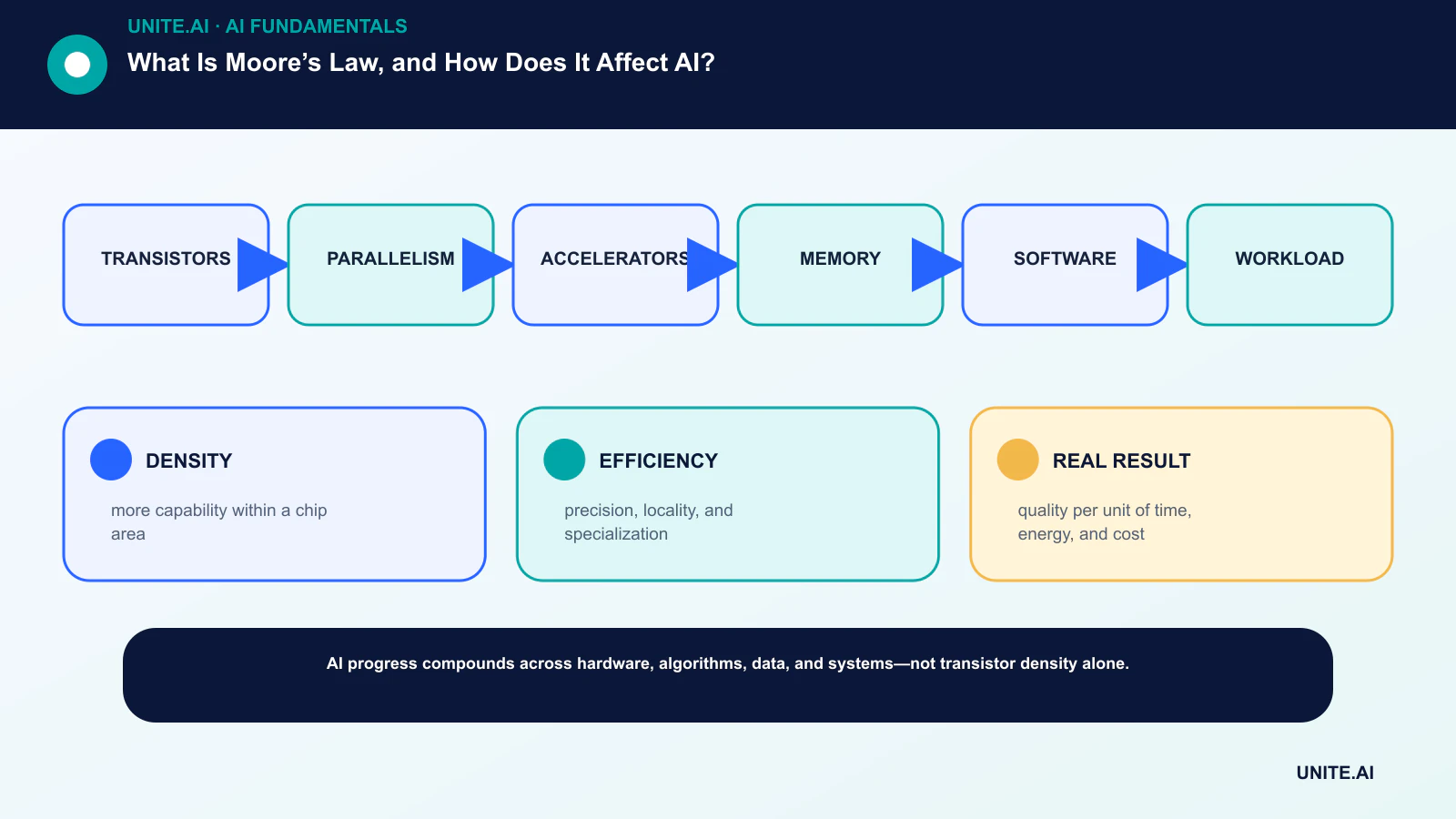
Turn the concept into a bounded, testable workflow: transistors → parallelism → accelerators → memory → software → workload. Name an accountable owner, document the data and dependencies, establish a simple baseline, set acceptance and stop criteria, test representative failures, and define monitoring, rollback, and review before expanding scope. Record versions and assumptions so another team can reproduce the result and understand what changed.

Before launch, run a documented readiness review with the people who build, operate, secure, and are affected by the system. Test normal cases, boundary conditions, dependency failures, and misuse; preserve the evidence and unresolved risks. Define who can approve release, change a threshold, override an output, or stop operation. Revisit the decision after real-world data arrives, because a technically successful pilot does not guarantee reliable performance at broader scale.

• DENSITY: more capability within a chip area.
• EFFICIENCY: precision, locality, and specialization.
• REAL RESULT: quality per unit of time, energy, and cost.

Frequently asked questions

Is Moore’s Law over?

The simple historical trend has slowed and changed character, but semiconductor progress continues through devices, architecture, packaging, memory, and software. Whether the phrase still fits depends on the metric.

Does twice as many transistors mean twice the AI performance?

No. Performance depends on how transistors are used and on bandwidth, precision, model structure, software efficiency, power, and workload constraints.

Primary references

• Gordon Moore: Cramming More Components onto Integrated Circuits
• IEEE IRDS: International Roadmap for Devices and Systems
• MLCommons: MLPerf Benchmarks